(Solved): Instructions: - Submit a report containing a detailed description of all the tasks. - Provide MATLAB ...

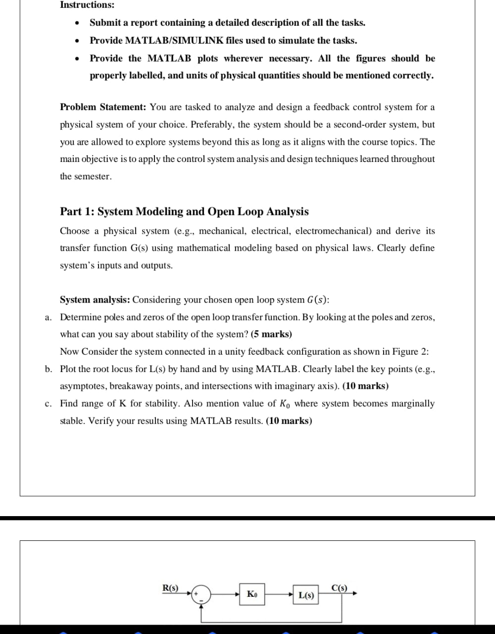
Instructions: - Submit a report containing a detailed description of all the tasks. - Provide MATLAB/SIMULINK files used to simulate the tasks. - Provide the MATLAB plots wherever necessary. All the figures should be properly labelled, and units of physical quantities should be mentioned correctly. Problem Statement: You are tasked to analyze and design a feedback control system for a physical system of your choice. Preferably, the system should be a second-order system, but you are allowed to explore systems beyond this as long as it aligns with the course topics. The main objective is to apply the control system analysis and design techniques learned throughout the semester. Part 1: System Modeling and Open Loop Analysis Choose a physical system (e.g., mechanical, electrical, electromechanical) and derive its transfer function G(s) using mathematical modeling based on physical laws. Clearly define system's inputs and outputs. System analysis: Considering your chosen open loop system \( G(s) \) : a. Determine poles and zeros of the open loop transfer function. By looking at the poles and zeros, what can you say about stability of the system? ( \( \mathbf{5} \) marks) Now Consider the system connected in a unity feedback configuration as shown in Figure 2: b. Plot the root locus for L(s) by hand and by using MATLAB. Clearly label the key points (e.g., asymptotes, breakaway points, and intersections with imaginary axis). ( \( \mathbf{1 0} \) marks) c. Find range of K for stability. Also mention value of \( K_{0} \) where system becomes marginally stable. Verify your results using MATLAB results. ( \( \mathbf{1 0} \) marks) solve it according to spring mass system second order syetem example